Changes values within a specified range, or greater than or less than a specific value to a new value in a vector, data.frame, or raster
Source:R/general_range_to_new_value.R
range_to_new_value.RdThis function modifies values in the input object x based on the specified
conditions. It can operate on vectors, data.frames, or RasterLayer objects.
The function allows for changing values within a specified range (between),
greater than or equals to (greater_than) or less than or equals to
(less_than) a specified value to a new value (new_value). An option to
invert the selection is also available for ranges.
Usage
range_to_new_value(
  x = NULL,
  between = NULL,
  greater_than = NULL,
  less_than = NULL,
  new_value = NULL,
  invert = FALSE
)
Arguments
- x
A numeric
vector,data.frame,RasterLayer,SpatRaster, orPackedSpatRasterobject whose values are to be modified.- between
Numeric. A numeric vector of length 2 specifying the range of values to be changed or kept. If specified,
greater_thanandless_thanare ignored.- greater_than, less_than
Numeric. Threshold larger than or equal to/less than or equal to which values in
xwill be changed tonew_value. Only applied ifbetweenis not specified.- new_value
The new value to assign to the selected elements in
x.- invert
Logical. Whether to invert the selection specified by
between. IfTRUE, values outside the specified range are changed tonew_value. Default isFALSE.
Examples
ecokit::load_packages(dplyr, raster, terra, tibble, ggplot2, tidyr)
# ---------------------------------------------
# Vector
(VV <- seq_len(10))
#> [1] 1 2 3 4 5 6 7 8 9 10
range_to_new_value(x = VV, between = c(5, 8), new_value = NA)
#> [1] 1 2 3 4 NA NA NA NA 9 10
range_to_new_value(x = VV, between = c(5, 8), new_value = NA, invert = TRUE)
#> [1] NA NA NA NA 5 6 7 8 NA NA
# greater_than is ignored as `between` is specified
range_to_new_value(
x = VV, between = c(5, 8), new_value = NA, greater_than = 4)
#> [1] 1 2 3 4 NA NA NA NA 9 10
range_to_new_value(x = VV, new_value = NA, greater_than = 4)
#> [1] 1 2 3 NA NA NA NA NA NA NA
range_to_new_value(x = VV, new_value = NA, less_than = 4)
#> [1] NA NA NA NA 5 6 7 8 9 10
# `invert` argument works only when `between` is specified
range_to_new_value(x = VV, new_value = NA, greater_than = 4, invert = TRUE)
#> [1] 1 2 3 NA NA NA NA NA NA NA
# ---------------------------------------------
# tibble
iris2 <- iris %>%
tibble::as_tibble() %>%
dplyr::slice_head(n = 50) %>%
dplyr::select(-Sepal.Length, -Petal.Length, -Petal.Width) %>%
dplyr::arrange(Sepal.Width)
iris2 %>%
dplyr::mutate(
Sepal.Width.New = range_to_new_value(
x = Sepal.Width, between = c(3, 3.5),
new_value = NA, invert = FALSE),
Sepal.Width.Rev = range_to_new_value(
x = Sepal.Width, between = c(3, 3.5),
new_value = NA, invert = TRUE)) %>%
print(n = 50)
#> # A tibble: 50 × 4
#> Sepal.Width Species Sepal.Width.New Sepal.Width.Rev
#> <dbl> <fct> <dbl> <dbl>
#> 1 2.3 setosa 2.3 NA
#> 2 2.9 setosa 2.9 NA
#> 3 3 setosa NA 3
#> 4 3 setosa NA 3
#> 5 3 setosa NA 3
#> 6 3 setosa NA 3
#> 7 3 setosa NA 3
#> 8 3 setosa NA 3
#> 9 3.1 setosa NA 3.1
#> 10 3.1 setosa NA 3.1
#> 11 3.1 setosa NA 3.1
#> 12 3.1 setosa NA 3.1
#> 13 3.2 setosa NA 3.2
#> 14 3.2 setosa NA 3.2
#> 15 3.2 setosa NA 3.2
#> 16 3.2 setosa NA 3.2
#> 17 3.2 setosa NA 3.2
#> 18 3.3 setosa NA 3.3
#> 19 3.3 setosa NA 3.3
#> 20 3.4 setosa NA 3.4
#> 21 3.4 setosa NA 3.4
#> 22 3.4 setosa NA 3.4
#> 23 3.4 setosa NA 3.4
#> 24 3.4 setosa NA 3.4
#> 25 3.4 setosa NA 3.4
#> 26 3.4 setosa NA 3.4
#> 27 3.4 setosa NA 3.4
#> 28 3.4 setosa NA 3.4
#> 29 3.5 setosa NA 3.5
#> 30 3.5 setosa NA 3.5
#> 31 3.5 setosa NA 3.5
#> 32 3.5 setosa NA 3.5
#> 33 3.5 setosa NA 3.5
#> 34 3.5 setosa NA 3.5
#> 35 3.6 setosa 3.6 NA
#> 36 3.6 setosa 3.6 NA
#> 37 3.6 setosa 3.6 NA
#> 38 3.7 setosa 3.7 NA
#> 39 3.7 setosa 3.7 NA
#> 40 3.7 setosa 3.7 NA
#> 41 3.8 setosa 3.8 NA
#> 42 3.8 setosa 3.8 NA
#> 43 3.8 setosa 3.8 NA
#> 44 3.8 setosa 3.8 NA
#> 45 3.9 setosa 3.9 NA
#> 46 3.9 setosa 3.9 NA
#> 47 4 setosa 4 NA
#> 48 4.1 setosa 4.1 NA
#> 49 4.2 setosa 4.2 NA
#> 50 4.4 setosa 4.4 NA
# ---------------------------------------------
# RasterLayer
grd_file <- system.file("external/test.grd", package = "raster")
R_raster <- raster::raster(grd_file)
# set the theme for ggplot2
ggplot2::theme_set(
ggplot2::theme_minimal() +
ggplot2::theme(
legend.position = "right",
strip.text = ggplot2::element_text(size = 16),
legend.title = ggplot2::element_blank(),
axis.title = ggplot2::element_blank(),
axis.text = ggplot2::element_blank()))
# Convert values less than 500 to NA
R_raster2 <- range_to_new_value(
x = R_raster, less_than = 500, new_value = NA)
# Convert values greater than 600 to NA
R_raster3 <- range_to_new_value(
x = R_raster, greater_than = 600, new_value = NA)
(R_rasters <- raster::stack(R_raster, R_raster2, R_raster3))
#> class : RasterStack
#> dimensions : 115, 80, 9200, 3 (nrow, ncol, ncell, nlayers)
#> resolution : 40, 40 (x, y)
#> extent : 178400, 181600, 329400, 334000 (xmin, xmax, ymin, ymax)
#> crs : +proj=sterea +lat_0=52.1561605555556 +lon_0=5.38763888888889 +k=0.9999079 +x_0=155000 +y_0=463000 +datum=WGS84 +units=m +no_defs
#> names : test.1, test.2, test.3
#> min values : 138.7071, 500.1736, 138.7071
#> max values : 1736.0579, 1736.0580, 599.6334
#>
as.data.frame(R_rasters, xy = TRUE, na.rm = FALSE) %>%
stats::setNames(c("x", "y", "R_raster", "R_raster2", "R_raster3")) %>%
tidyr::pivot_longer(
cols = -c("x", "y"), names_to = "layer", values_to = "value") %>%
ggplot2::ggplot() +
ggplot2::geom_tile(mapping = ggplot2::aes(x = x, y = y, fill = value)) +
ggplot2::facet_grid(~layer) +
ggplot2::scale_fill_gradientn(
colours = c("blue", "green", "yellow", "red"),
na.value = "transparent") +
ggplot2::labs(title = NULL, x = NULL, y = NULL) +
ggplot2::coord_cartesian(expand = FALSE, clip = "off")
 # ---------------------------------------------
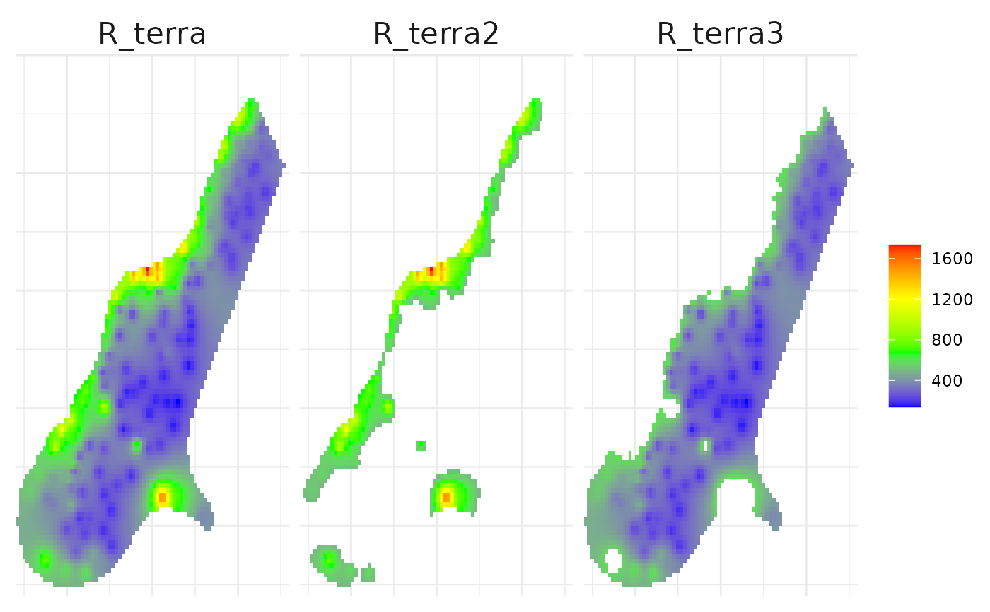
# SpatRaster
R_terra <- terra::rast(grd_file)
R_terra2 <- range_to_new_value(x = R_terra, less_than = 500, new_value = NA)
R_terra3 <- range_to_new_value(
x = R_terra, greater_than = 600, new_value = NA)
(R_terras <- c(R_terra, R_terra2, R_terra3))
#> class : SpatRaster
#> size : 115, 80, 3 (nrow, ncol, nlyr)
#> resolution : 40, 40 (x, y)
#> extent : 178400, 181600, 329400, 334000 (xmin, xmax, ymin, ymax)
#> coord. ref. : +proj=sterea +lat_0=52.1561605555556 +lon_0=5.38763888888889 +k=0.9999079 +x_0=155000 +y_0=463000 +datum=WGS84 +units=m +no_defs
#> sources : test.grd
#> spat_20fe5a45039a_8446_J0P2uAoeGj8eURN.tif
#> spat_20fe70094f1e_8446_omf5NvSmIUuRURk.tif
#> varnames : test
#> test
#> test
#> names : test, test, test
#> min values : 138.707073, 500.173645, 138.707077
#> max values : 1736.05793, 1736.057983, 599.633423
as.data.frame(R_terras, xy = TRUE, na.rm = FALSE) %>%
stats::setNames(c("x", "y", "R_terra", "R_terra2", "R_terra3")) %>%
tidyr::pivot_longer(
cols = -c("x", "y"), names_to = "layer", values_to = "value") %>%
ggplot2::ggplot() +
ggplot2::geom_tile(mapping = ggplot2::aes(x = x, y = y, fill = value)) +
ggplot2::facet_grid(~layer) +
ggplot2::scale_fill_gradientn(
colours = c("blue", "green", "yellow", "red"),
na.value = "transparent") +
ggplot2::labs(title = NULL, x = NULL, y = NULL) +
ggplot2::coord_cartesian(expand = FALSE, clip = "off")
# ---------------------------------------------
# SpatRaster
R_terra <- terra::rast(grd_file)
R_terra2 <- range_to_new_value(x = R_terra, less_than = 500, new_value = NA)
R_terra3 <- range_to_new_value(
x = R_terra, greater_than = 600, new_value = NA)
(R_terras <- c(R_terra, R_terra2, R_terra3))
#> class : SpatRaster
#> size : 115, 80, 3 (nrow, ncol, nlyr)
#> resolution : 40, 40 (x, y)
#> extent : 178400, 181600, 329400, 334000 (xmin, xmax, ymin, ymax)
#> coord. ref. : +proj=sterea +lat_0=52.1561605555556 +lon_0=5.38763888888889 +k=0.9999079 +x_0=155000 +y_0=463000 +datum=WGS84 +units=m +no_defs
#> sources : test.grd
#> spat_20fe5a45039a_8446_J0P2uAoeGj8eURN.tif
#> spat_20fe70094f1e_8446_omf5NvSmIUuRURk.tif
#> varnames : test
#> test
#> test
#> names : test, test, test
#> min values : 138.707073, 500.173645, 138.707077
#> max values : 1736.05793, 1736.057983, 599.633423
as.data.frame(R_terras, xy = TRUE, na.rm = FALSE) %>%
stats::setNames(c("x", "y", "R_terra", "R_terra2", "R_terra3")) %>%
tidyr::pivot_longer(
cols = -c("x", "y"), names_to = "layer", values_to = "value") %>%
ggplot2::ggplot() +
ggplot2::geom_tile(mapping = ggplot2::aes(x = x, y = y, fill = value)) +
ggplot2::facet_grid(~layer) +
ggplot2::scale_fill_gradientn(
colours = c("blue", "green", "yellow", "red"),
na.value = "transparent") +
ggplot2::labs(title = NULL, x = NULL, y = NULL) +
ggplot2::coord_cartesian(expand = FALSE, clip = "off")