Calculate Nearest Neighbour Distances for Spatial Features

This function calculates the nearest neighbour distance for each feature in an sf object. It rasterizes the input data at a specified resolution, converts to polygons, and then computes the distance to the nearest neighbour for each feature. The function can be used to detect spatial outliers before use in ecological modelling like species distribution models.

Usage

nearest_dist_sf(sf_object, resolution = 0.25, n_cores = 6L)

Arguments

sf_object: An sf object with CRS EPSG:4326. Must contain at least 2 features.
resolution: Numeric. The resolution for rasterization in degrees. Default is 0.25. Must be a single positive numeric value. The smaller the resolution, the more accurate the distance calculations, but also the more computationally intensive.
n_cores: Integer. The number of cores to use for parallel processing. Default is 6L.

Value

An sf object identical to the input sf_object with an additional column nearest_dist containing the distance (in kilometres) to the nearest neighbour for each feature.

Details

The function performs the following steps:

Validates that the input is an sf object with CRS EPSG:4326 and contains at least 2 features
Rasterizes the input data at the specified resolution
Converts raster cells to polygons
Calculates centroids for faster distance computation
Computes the distance to the second nearest neighbour (the first is the feature itself)
Joins the calculated distances back to the original sf object

Author

Ahmed El-Gabbas

Examples

# Create sample sf object
ecokit:::load_packages(sf, dismo, fs, dplyr, tibble, rworldmap, ggplot2)

occurrence <- system.file(package = "dismo") %>%
  fs::path("ex", "bradypus.csv") %>%
  read.table(header = TRUE, sep = ",") %>%
  tibble::tibble() %>%
  st_as_sf(crs = 4326L, coords = c("lon", "lat"))
head(occurrence)
#> Simple feature collection with 6 features and 1 field
#> Geometry type: POINT
#> Dimension:     XY
#> Bounding box:  xmin: -65.4 ymin: -17.45 xmax: -63.6667 ymax: -10.3833
#> Geodetic CRS:  WGS 84
#> # A tibble: 6 × 2
#>   species                        geometry
#>   <chr>                       <POINT [°]>
#> 1 Bradypus variegatus    (-65.4 -10.3833)
#> 2 Bradypus variegatus (-65.3833 -10.3833)
#> 3 Bradypus variegatus    (-65.1333 -16.8)
#> 4 Bradypus variegatus   (-63.6667 -17.45)
#> 5 Bradypus variegatus      (-63.85 -17.4)
#> 6 Bradypus variegatus      (-64.4167 -16)

# Calculate nearest distances
result <- nearest_dist_sf(occurrence, resolution = 0.25, n_cores = 2)
head(result)
#> Simple feature collection with 6 features and 2 fields
#> Geometry type: POINT
#> Dimension:     XY
#> Bounding box:  xmin: -65.4 ymin: -17.45 xmax: -63.6667 ymax: -10.3833
#> Geodetic CRS:  WGS 84
#> # A tibble: 6 × 3
#>   species                        geometry nearest_dist
#>   <chr>                       <POINT [°]>        <dbl>
#> 1 Bradypus variegatus    (-65.4 -10.3833)        645. 
#> 2 Bradypus variegatus (-65.3833 -10.3833)        645. 
#> 3 Bradypus variegatus    (-65.1333 -16.8)        115. 
#> 4 Bradypus variegatus   (-63.6667 -17.45)         26.6
#> 5 Bradypus variegatus      (-63.85 -17.4)         26.6
#> 6 Bradypus variegatus      (-64.4167 -16)        115. 

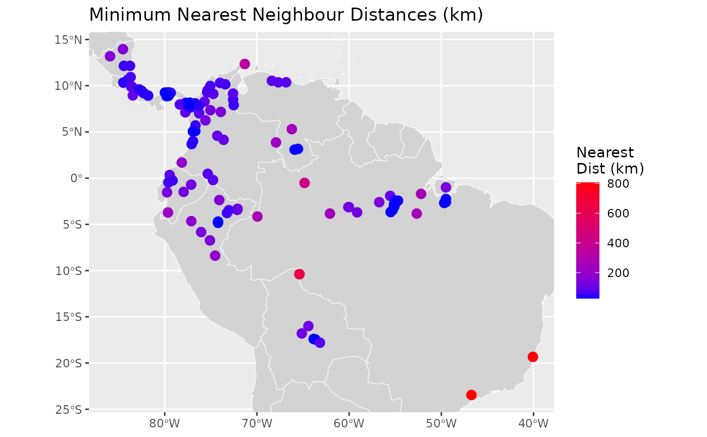
global_map <- sf::st_as_sf(rworldmap::getMap(resolution = "low"))

ggplot2::ggplot() +
  ggplot2::geom_sf(data = global_map, fill = "lightgray", color = "white") +
  ggplot2::geom_sf(
    data = result, ggplot2::aes(color = nearest_dist), size = 3) +
  ggplot2::scale_color_gradient(low = "blue", high = "red") +
  ggplot2::coord_sf(xlim = c(-85.9333, -40.0667), ylim = c(-23.45, 13.95)) +
  ggplot2::labs(
    title = "Minimum Nearest Neighbour Distances (km)",
    color = "Nearest\nDist (km)")