Mask raster to show top % and bottom % of cumulative sum
Source:R/eco_get_sampling_effort.R
mask_cumulative_pct.RdThis function complements the get_sampling_effort() function by creating
masked rasters that highlight areas contributing to the top and bottom
percentages of the cumulative sum of the original raster values. This can be
useful for identifying areas with the highest and lowest sampling efforts
based on the original raster (i.e., number of observations). The function
also identifies cells with zero observations. For more information, see this repo and El-Gabbas
(2026). DOI.
Value
A SpatRaster with three layers:
top_xx_percent_cumulative: cells cumulatively accounting for the toptop_pct%; wherexxis the value oftop_pctbottom_xx_percent_cumulative: cells cumulatively accounting for the lowest(100 - top_pct)%; wherexxis the value oftop_pctzero_observations: cells with original value equal to zero
Examples
require(terra)
temp_dir <- fs::path(fs::path_temp(), "sampling_efforts")
fs::dir_create(temp_dir)
# Sampling effort raster for birds (number of observations at 20 km
# resolution)
efforts_birds_all <- get_sampling_effort(
group = "aves", metric = "n_obs", resolution = 20, out_dir = temp_dir)
efforts_birds_all_r <- terra::rast(efforts_birds_all$local_path)
result <- mask_cumulative_pct(rast = efforts_birds_all_r, top_pct = 90)
result
#> class : SpatRaster
#> size : 1080, 2160, 3 (nrow, ncol, nlyr)
#> resolution : 0.1666667, 0.1666667 (x, y)
#> extent : -180, 180, -90, 90 (xmin, xmax, ymin, ymax)
#> coord. ref. : lon/lat WGS 84 (EPSG:4326)
#> source(s) : memory
#> varname : n_obs_Aves_res_20
#> names : top_90_per~cumulative, lowest_10_~cumulative, zero_observations
#> min values : 11303, 1, 1
#> max values : 6193941, 11303, 1
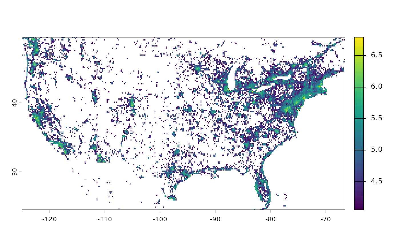
# Areas contributing to the top 90% of cumulative sum (log10 scale; computed
# on the global scale and cropped to USA)
result$top_90_percent_cumulative %>%
terra::crop(terra::ext(-125, -66.5, 24.5, 49.5)) %>%
log10() %>%
plot()
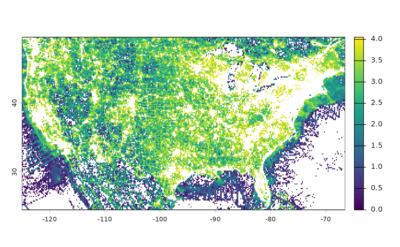
 # Areas contributing to the lowest 10% of cumulative sum (log10 scale;
# computed on the global scale and cropped to USA)
result$lowest_10_percent_cumulative %>%
terra::crop(terra::ext(-125, -66.5, 24.5, 49.5)) %>%
log10() %>%
plot()
# Areas contributing to the lowest 10% of cumulative sum (log10 scale;
# computed on the global scale and cropped to USA)
result$lowest_10_percent_cumulative %>%
terra::crop(terra::ext(-125, -66.5, 24.5, 49.5)) %>%
log10() %>%
plot()
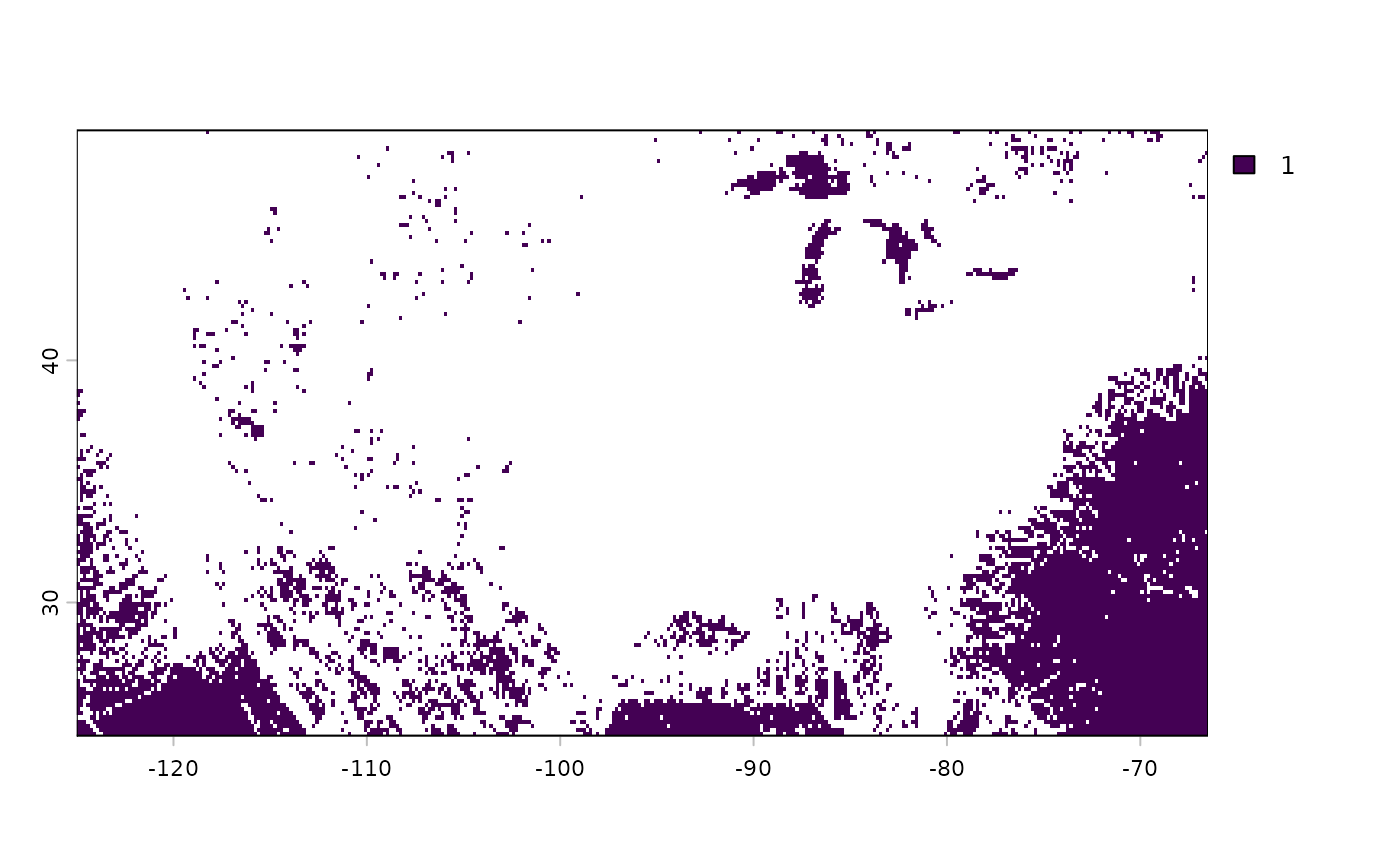
 # Areas with zero observations (computed on the global scale and cropped to
# USA)
result$zero_observations %>%
terra::crop(terra::ext(-125, -66.5, 24.5, 49.5)) %>%
plot()
# Areas with zero observations (computed on the global scale and cropped to
# USA)
result$zero_observations %>%
terra::crop(terra::ext(-125, -66.5, 24.5, 49.5)) %>%
plot()
 fs::dir_delete(temp_dir)